on
Blog 2: The Economy
This blog is an ongoing assignment for Gov 1347: Election Analytics, a course at Harvard College taught by Professor Ryan Enos. It will be updated weekly and culminate in a predictive model of the 2022 midterm elections.
“It’s the economy, stupid,” became a slogan of Bill Clinton’s 1992 presidential campaign. With the nation facing recession under incumbent President George H.W. Bush, political strategist James Carville coined the phrase to keep the campaign focused on the big picture. This notion that the economy is paramount is not only the subject of pithy sound bites, but also the basis of statistical models. Econometrician Ray Fair has been predicting elections since 1978 using only economic inputs. Political scientist Alan Abramowitz’s noted straightforward “Time For Change” model uses GDP as one of its three variables. Thus, in this second blog post, I’ll present my first models of the 2022 midterms, based solely on national economic data. I will complete blog extensions 1 and 2.
It’s impossible to disentangle the economy from incumbency. Obviously, in presidential elections, the incumbent is on the ballot and will be judged for his or her handling of the economy. But midterm elections are also often viewed as referendums on the incumbent president. Thus, for the following election models, I will predict the vote and seat share of the incumbent president’s party in the House of Representatives based on economic variables, including data from both presidential and midterm cycles. If the conventional wisdom holds, we should expect poor economic performance to coincide with bad results for the president’s party in House elections.
Real Disposable Income
I’ll begin by using change in real disposable income to predict House election results. One key question when using economic data to determine voter behavior is how far back we should look. In theory, if members of the electorate do vote based on how the president and his or her party have handled the economy, we should include 2-4 years of economic data to consider the president’s full tenure. But, as Andrew Healy and Gabriel S. Lenz demonstrate, short-term economic indicators often cloud out larger economic trends in voters’ minds. In their book Democracy for Realists, Christopher Achen and Larry Bartels model presidential elections based on real disposable income — along with a host of other variables. They find that short term growth in real disposable income over the last financial quarter before the election is a better predictor of the incumbent presidential popular vote than total income growth over the course of most of the four-year term.
In the models below, I will split the difference: use the growth in real disposable income from one year in advance of the election by comparing income in the third quarter of the election year and the third quarter of the year prior. The following scatterplot compares the annual growth in real disposable income in the year before the election with the House popular vote of the incumbent president’s party.
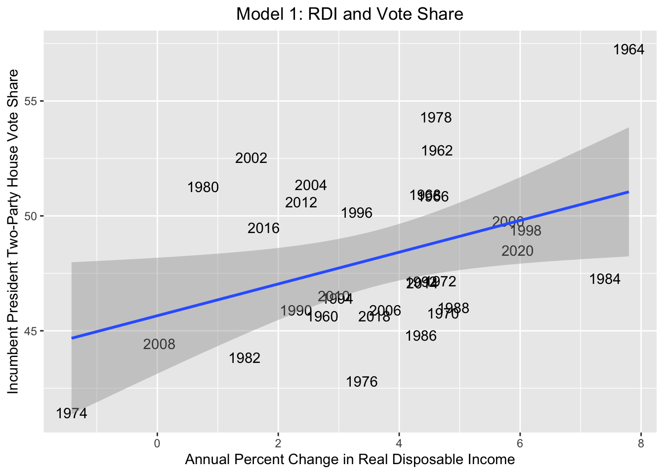
Below is the regression table for the relationship between real disposable income and House vote share of the incumbent president’s party.
| incumbent pres majorvote | ||||
|---|---|---|---|---|
| Predictors | Estimates | std. Error | CI | p |
| (Intercept) | 45.66 | 1.23 | 43.13 – 48.18 | <0.001 |
| DSPIC change pct yearly | 0.69 | 0.30 | 0.08 – 1.30 | 0.028 |
| Observations | 31 | |||
| R2 / R2 adjusted | 0.157 / 0.128 | |||
Next, I’ll conduct the same model, but with House seat share rather than vote share as the dependent variable. The scatterplot is shown below.
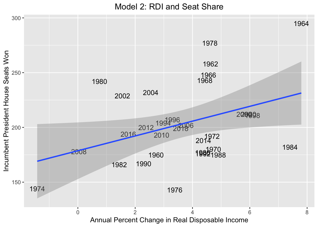
The regression table for this model is shown below.
| incumbent pres seats | ||||
|---|---|---|---|---|
| Predictors | Estimates | std. Error | CI | p |
| (Intercept) | 178.69 | 12.65 | 152.81 – 204.57 | <0.001 |
| DSPIC change pct yearly | 6.76 | 3.05 | 0.51 – 13.00 | 0.035 |
| Observations | 31 | |||
| R2 / R2 adjusted | 0.144 / 0.115 | |||
There are a few key takeaways from these models. First, as expected, there is a positive relationship between annual disposable income growth in the run-up to the election and the electoral performance of the incumbent president’s party. However, these relationships are not very strong — the relatively low R-squared values suggest that annual income growth is only somewhat predictive of electoral outcomes. The root-mean-square errors for the vote and seat models are 3.188 and 32.696, respectively. And over a series of cross-validation simulations, the mean absolute errors are 3.035 and 28.860, respectively. These errors are fairly large considering the close vote and seat margins that often decide control of the House.
So while it is clear that these simple bivariate models are far from perfect, we can still use them to develop predictions for the 2022 midterms. Unfortunately, the data input used to test these models is unavailable, as 2022’s third economic quarter is not yet over. But we can use the real disposable income change from the first quarter of 2021 to the first quarter of 2022 to get an estimate for the model’s input. Real disposable income actually shrunk by 12 percentage points from the first quarter of 2021 to the first quarter of 2022, and the models thus predict disastrous results for incumbent President Joe Biden’s Democratic Party. Per the two models, Democrats would only win around 37% of the two-party vote and only around 98 seats. These outcomes are obviously quite extreme, requiring a nearly total collapse in Democratic support. Still, these predictions align with the broader economic theory surrounding this election: a bad economy will be bad for Democrats.
Notably, the seats model is more extreme than the votes model: 37% of the vote corresponds to around 160 seats, far greater than the 98 seats predicted by the seats model. This could suggest that seat share swings more violently with economic trends than vote share does.
Gross Domestic Product
I’ll use the same approach to predict House seat and vote shares with GDP. The models below forecast election results based on GDP growth between the third quarter of the year before the election and the third quarter of the election year. The scatterplot below uses vote share as the dependent variable.
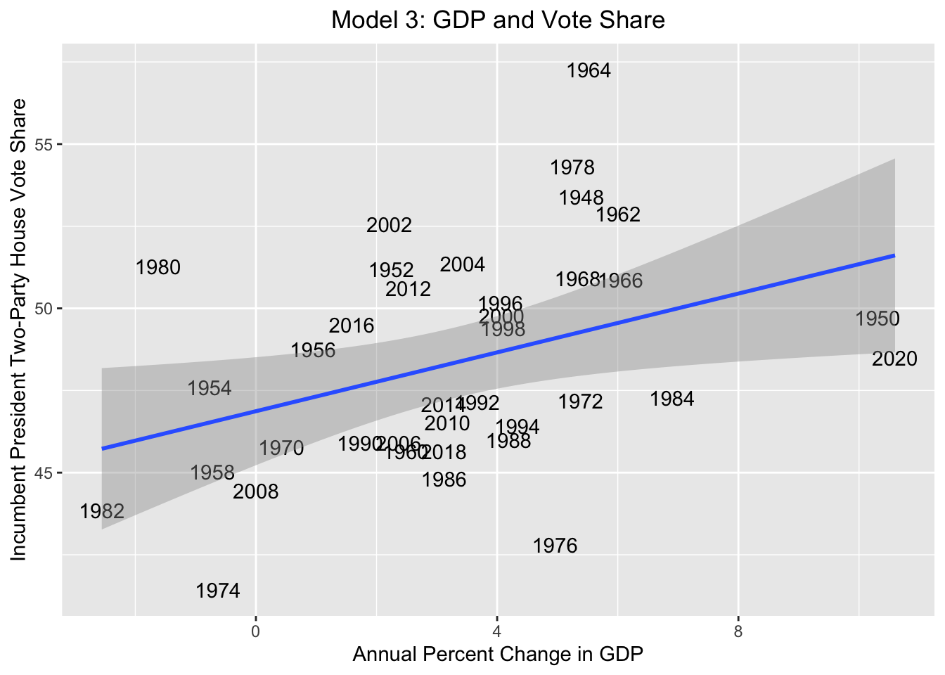
Below is the regression output.
| incumbent pres majorvote | ||||
|---|---|---|---|---|
| Predictors | Estimates | std. Error | CI | p |
| (Intercept) | 46.87 | 0.81 | 45.23 – 48.51 | <0.001 |
| GDPC1 growth pct yearly | 0.45 | 0.19 | 0.07 – 0.82 | 0.021 |
| Observations | 37 | |||
| R2 / R2 adjusted | 0.142 / 0.118 | |||
The next model predicts the House seat share of the incumbent party’s president based on annual GDP growth.
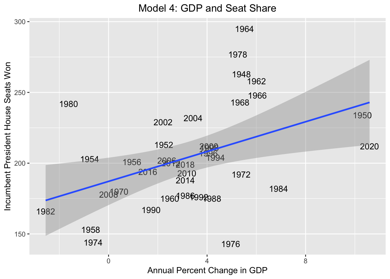
Below is the regression table.
| incumbent pres seats | ||||
|---|---|---|---|---|
| Predictors | Estimates | std. Error | CI | p |
| (Intercept) | 187.13 | 8.25 | 170.39 – 203.88 | <0.001 |
| GDPC1 growth pct yearly | 5.27 | 1.89 | 1.43 – 9.11 | 0.009 |
| Observations | 37 | |||
| R2 / R2 adjusted | 0.181 / 0.158 | |||
Once again, as expected, there appears to be a positive relationship between annual GDP growth and the president’s party’s performance in the House. Still, the relationships remain fairly weak, as judged by the R-squared values. The root-mean-square errors for the vote and seat models are 3.126 and 31.838, respectively. The mean absolute errors derived from cross-validation simulations are 2.876 and 26.695, respectively.
Clearly, annual GDP growth does not tell the full story of why parties perform well or poorly in House elections, but we can still use our models to generate predictions. I’ll again turn to GDP data from the first quarter of 2021 and the first quarter of 2022 to determine an estimate for annual GDP growth. GDP actually grew by around 10.7%, and as a result of this strong economic growth, these models show Joe Biden’s Democrats winning the House. Democrats are predicted to win around 51.6% of the House popular vote and 243 seats. This strong performance for the Democrats runs directly counter to the results of my RDI model.
Once again, using seat share as the dependent variable seems to predict more extreme results. 51.6% of the popular vote corresponds to around 225 seats, less than 243. This again could suggest that seat share is more responsive than the popular vote to broad economic trends.
Conclusion
Ultimately, I am quite skeptical of these models. The low R-squared values and high error indicators suggest that annual RDI and GDP only loosely fit the House election data. The following residual plots, with the predicted results represented by dots and actual results represented by lines, similarly demonstrate the imprecision of the models.
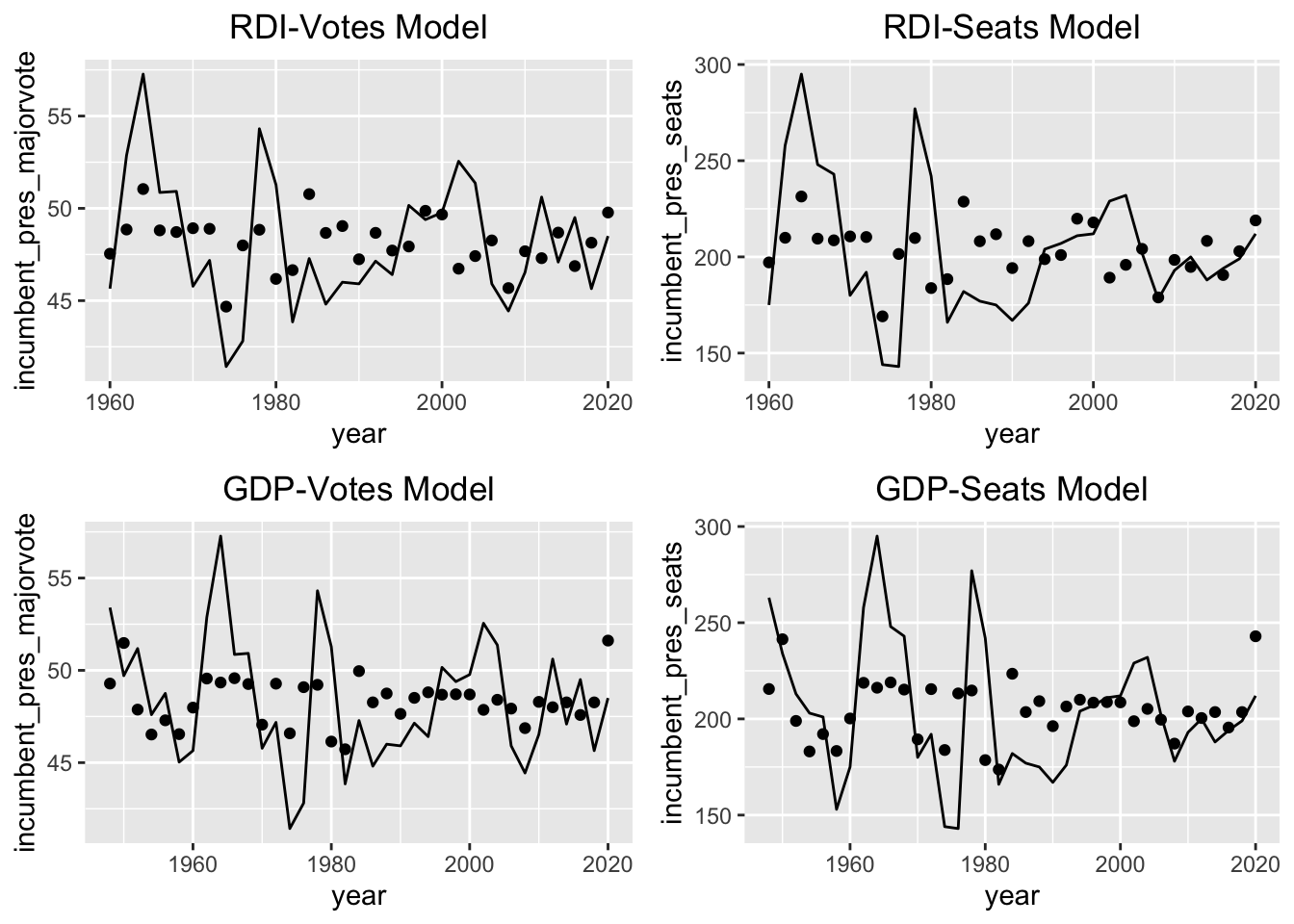
Of course, it is not surprising that these models are inexact. If one or two broad economic indicators could super accurately predict election results, it would be a lot easier to forecast elections. Still, there are some important lessons from this exercise. The linear models explored above do demonstrate that, broadly speaking, the incumbent president’s party tends to fare better in the House when the economy is doing well. But the specific measure used to assess the state of the economy can have a drastic impact on our predictions. The model based on real disposable income produced a nearly opposite prediction compared to our model based on GDP. As I continue to refine my predictions, I’ll thus be certain to consider a range of different variables — both economic and otherwise — when constructing my models.